Prometheus S&P 500 Program Primer

Launch Discount: 38% Off. Ends Soon.

We started Prometheus with a simple premise: bring the highest quality of institutional-grade macro investment research to everyday investors. Today, we are taking another big step in this direction with the official launch of our systematic Prometheus S&P 500 Program.

To help investors through these volatile times, we began sharing the positions from this program earlier this year. Today, we release the complete primer for the program. In the spirit of the program’s official release, we are offering a one-time discount of 38% on our monthly price for annual subscribers. You can avail of this offer at the link below. The offer will expire very soon.

The Prometheus S&P 500 Program aims to outperform the S&P 500 over a full investment cycle. The program will aim to achieve this objective by leveraging a combination of Sector Selection, Beta Timing, Active Overlays, and Dynamic Risk Control.

The program trades the following assets:

• S&P 500: SPY/E-mini Futures/SPXU/SPXS (Long & Short Exposure)

• Industrials: XLI (Long Only)

• Technology: XLK (Long Only)

• Homebuilders: XHB or ITB (Long Only)

• Treasuries: TYA, TUA (Long Only)

The program rotates between these assets weekly, with updates on Mondays between 3:30 and 4:00 PM ET. You can download the complete primer using the link below or read it in the body of this note.

Prometheus S&P 500 Program: Primer

1.42MB ∙ PDF file

Download

Download

The primer aims to develop a robust understanding of the Prometheus S&P 500 Program. Even if you choose not to follow the program, the portfolio construction framework will offer valuable and structured insights into our answer to the question: How Do You Beat The Stock Market?

Let’s dive in.

Prometheus S&P 500 Program: Primer

The S&P 500 has become the world's preeminent equity benchmark for US and global investors. While passive exposure to the S&P 500 has served investors well in the past, we think we can use our suite of macro tools to improve that allocation and create something better in the form of our Prometheus S&P 500 Program.

The US equity market has far outperformed its peers globally and most active managers domestically. Since 2010, the S&P 500 has provided investors with a return-to-risk profile consistent with those of a sophisticated asset manager, generating 13.3% annualized returns over cash at 17.2% volatility, i.e., a Sharpe Ratio of 0.78. Given the conservative nature of most institutional investors, even if they have matched or somewhat outperformed this risk-adjusted return, they were unlikely to have maintained such a high volatility profile, leading to underperformance. Combining these risk-adjusted and absolute return characteristics with the proliferation of low-cost ETFs, the S&P 500 has become the primary benchmark against which most investors measure success.

We think it is unlikely that equities can continue to perform at this pace over the long term. Over a very long history, beginning in the 1900s, the equity market has had a Sharpe Ratio closer to 0.35, i.e., about half of what we have seen since 2010. That is our long-term expectation. However, how that long-term expectation comes to fruition is a question whose answer extends beyond the capabilities of reasonable quantitative investing. We may have another two decades of exceptional equity returns followed by a lost decade, a re-run of the technology bubble, followed by an extraordinary bust, or any one of the infinite number of permutations of the future. Those long-term future paths are unknowable, and any strategy that seeks to bet on such long-term paths is much closer to a coin flip than a durable investment strategy in its odds of success. US equity market dominance is here to stay, at least for a while.

Given the centrality of US equity markets today, we think it is our role as active investors to seek to add value to this core component of investor portfolios. If most investors seek equity-like exposure, we think it’s our job to add an edge to that exposure. We believe that with a combination of security selection, macro timing, active diversification, and tight risk management, investors can outperform the equity market significantly over a full investment cycle.

Crucially, we don’t think it is possible to outperform every week, month, or even year. However, with a consistent and disciplined approach, we believe it is possible to harness most of the upside in equities while ameliorating or avoiding the downside. We think the outperformance generated through the successful implementation of this process will materialize over the course of a full investment cycle. We define a full investment cycle as an investment cycle where markets have experienced bull and bear markets with a generalized upward drift.

We think we can pull four big portfolio construction levers to create durable outperformance versus the S&P 500 over a full investment cycle. We visualize our process below:

We think pulling these levers can create a portfolio that seeks to maintain significant upside capture in bull markets and limited or short exposure in bear markets while maintaining a much more moderate drawdown profile compared to the benchmark. As always, our systematic approach has allowed us to simulate the strategy's performance far back in history, allowing us to deeply assess the durability of our approach and learn from history. In this primer, we describe the mechanics underlying the investment process to help develop a better understanding of what to expect for those who choose to follow the strategy. We dive into each of the levers and their simulations, beginning with Sector Selection.

Sector Selection: Offsetting Inflation Shocks

Sector Selection seeks to find relative value opportunities within equity sectors and profit from those opportunities by rotating between sectors. The prerequisite for such rotation to be successful is adequate dispersion between sectors. However, the dispersion between equity sectors is quite low over time. This does not mean that there aren’t regimes of significant dispersion, but that dispersion is a sporadic rather than a persistent one. Below, we visualize the distribution of Sharpe Ratios (excess return over volatility) for equity sectors since 1965:

We see this relatively uniform distribution of outcomes even during recessions:

This lack of dispersion amongst sector returns is broadly consistent with a relatively uniform pass-through of economic growth to equity prices.

At the index level, the most dominant driver of changes to the equity market is changes in growth expectations, which flow through to earnings expectations, which flow through to the index, and then various sectors. We find that responsiveness to big growth-induced moves is uniform in terms of their price impact on sectors. As such, only modest alpha can be achieved by rotating based on growth conditions.

However, we find that considerably more information is available in the distribution of profits in the economy. The most significant shocks to this distribution of profits come from inflation shocks, which redistribute income between sectors rapidly. Some sectors are mechanically better suited to benefit from inflationary surges than others, particularly inflation beneficiaries. We can estimate the inflationary shocks relevant to the cross-section of equity returns using fundamental and price-based data. We visualize this proprietary gauge below:

During periods of elevated inflationary pressures, as quantified above, we see much more significant sector dispersion:

As we can see, inflation shocks create significantly more dispersion of equity returns relative to their typically uniform distribution. Applying this understanding, our Prometheus S&P 500 Program seeks to rotate based upon inflationary conditions to sectors best suited to profit from the current backdrop. For simplicity of execution, our program will rotate between four sectors, holding two at any given time: technology, industrials, homebuilders, and energy. We visualize how this process of equity sector rotation can add significant value as compared to passive exposure to the S&P 500 on a volatility-matched basis:

Above, we show how this sector selection process modestly improves all portfolio return and risk measures. Choosing equity sectors positioned to benefit from the distribution of nominal spending in the form of inflationary shocks improves portfolio Sharpe, Sortino, and Calmar Ratios, and reduces drawdown magnitude and duration. Though these improvements are modest, they offer meaningful benefits when combined with our other portfolio construction levers. The primary shortcoming of this strategy is that while it seeks to add a modest amount of returns by capitalizing on dispersion within sectors, it does not protect the portfolio from periods when moves across sectors are highly correlated. As stated differently, sector selection alone does not account for beta. This recognition brings us to our next portfolio construction lever: Beta Timing.

Beta Timing: Macro Drives Carry, Trend & Reversion

Beta Timing is the most proprietary component of our process, coming from our institutional alpha programs. To protect our edge in markets, we cannot share the formulas and techniques we use to try to predict the direction of markets. However, we can share the conceptual mechanics that drive our approach. At the core of our alpha generation process is a fundamental understanding of the nature of asset price returns. Every asset (stocks, bonds, commodities) carries an expected return for a given level of risk. This return can come through one of two ways: the asset can generate a cash flow for simply holding it, like an interest payment or a dividend, or the asset's price can change. If an asset generates positive returns for merely holding it, it has a positive carry. By and large, the most preferable assets to own over the long term are assets that offer a reasonable carry relative to their risk. In addition to carry, an asset may offer returns via its appreciation. This price appreciation can come in one of two ways: prices can rise after a recent fall (mean reversion) or after a recent gain (trend). To generate alpha, an investor needs a forward-looking view of the carry of the asset and whether its price will mean-revert or trend. At Prometheus, we think that macroeconomic forces dominate the intersection of these forces to determine whether carry, trend, or reversion will explain future returns.

Macroeconomic conditions determine whether carry, trend, or reversion will dominate the future returns of an asset.

Macroeconomic conditions determine whether carry, trend, or reversion will dominate the future returns of an asset.

We show some examples of these relationships below. During a downtrend in equity markets, whether they bounce (mean revert) or fall further (trend) is dependent on whether we are in a business cycle expansion or a recession:

As another example of this macro dominance, we show how carry is attractive in treasury markets primarily outside monetary policy hiking cycles:

For structural reasons, macro markets are replete with these relationships, allowing us to create investment strategies geared towards harnessing these predictive relationships.

Our research process is built around understanding these cause-and-effect relationships to create a dynamic and balanced exposure to carry, trend, and mean reversion based on macro conditions to manage the macro risks to equity markets.

The primary risk that all equities are exposed to is the risk of a persistent and pervasive economic contraction, i.e., a recession. Secondarily, equities are often at risk of more minor corrections when they have become rich versus bonds, commodities, and cash in a manner inconsistent with their fundamental economic drivers. These risk factors contribute to both the upside and downside risk, i.e., they can cause equity returns to deviate from their long-term mean returns, upwards and downwards. For a nimble and adaptive macro strategy, these deviations offer opportunities to add alpha uncorrelated to the long-term trajectory of the equity market. Our systematic macro process consistently evaluates the probability of these outcomes to trade equities long and short— we call this Beta Timing. Our Beta Timing Program seeks to use macro tools to ride trends and mean reversion opportunities in a dynamic fashion based on the evolving opportunity set. We visualize how, at times, our Beta Timing measures will be in line with macro trends, but at times meaningfully from trends to bet on mean reversion:

Crucially, this process is mechanically and empirically uncorrelated with the underlying market and depends entirely on whether our systems can anticipate what’s likely to transpire. We can use these signals to achieve higher confidence in whether equity markets will likely outperform or underperform. We can take these quantitative estimates of over/underperformance to estimate potential returns and use them to lever up or scale down our equity exposure. When equities are cheap and the economy is expanding, these signals dial up portfolio exposure. Conversely, when equities are expensive and the economy is at risk of a recession, these signals may take equity exposure to zero or even enter a net-short position.

Below, we visualize the portfolio improvements achieved through this Beta Timing:

Adding this layer of Beta Timing to our Sector Selection process is extremely accretive to total portfolio performance. This process boosts all risk-adjusted return measures, reducing drawdown depth and duration. As previously mentioned, the systems that drive our beta timing process are the proprietary output of our systematic process. However, the intuition of our Beta Timing Strategy is straightforward:

Our Beta Timing program will seek to balance exposures to carry, trend, and mean reversion, capitalizing on whichever signals offer us the most ex-ante alpha potential. When equities are rich versus macroeconomic conditions and near-term trends are conducive to short exposures, our systems will seek to short equity markets. Conversely, our systems will seek to buy equities aggressively when equity markets are cheap relative to macroeconomic conditions and near-term trends support long exposures.

We think the combination of Sector Selection and Beta Timing offers a better alternative to traditional passive exposure to the S&P 500 by improving an equity portfolio's resilience to inflation shocks and exploiting local cheapness and richness. However, this dynamic exposure to equities creates a significant average cash allocation over time, allowing us to overlay other strategies on the portfolio. We turn to this lever next.

Strategy Overlays: Active Treasury Strategy

Combining Sector Selection and Beta Timing creates a return stream that consistently changes its total exposure to equities. When there is a lot of signal, there is a lot of exposure. When there is little signal, the systems maintain very modest exposures. We cannot know how these signals will be distributed over the next few months or years. Often, our signals may dial down their exposure, taking significantly less volatility than the S&P 500. Traditionally, this decrease in exposure would increase cash positions.

However, we can further enhance portfolio returns by investing that cash actively in bonds. These overlays aim to achieve more effective cash utilization during times of lower equity market exposures. This approach allows us to ensure we do not have excessive drift from the benchmark but can also reliably add returns above cash to the portfolio, further boosting the potential for long-term outperformance. We find these overlays extremely additive when our strategies have begun to reduce exposures, but equity markets may continue to power ahead. Alternatively, when our bets have low conviction and may run the risk of being offside, these additional exposures serve as diversification. The excess returns generated through these overlays help bolster the portfolio’s returns, allowing total returns to maintain pace with the benchmark without excessively loading on equity market risk at inopportune periods.

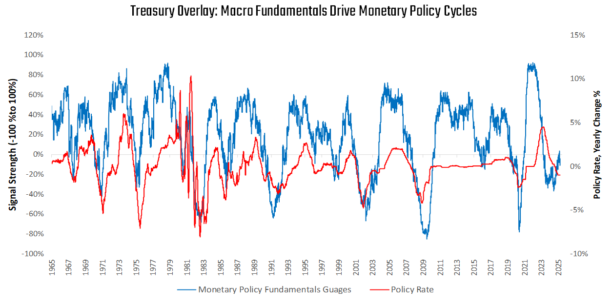
It is crucial to note that an active investment process is integral to the success of this overlay. Treasury securities have had a long history as a strong diversifier to stocks. However, treasuries come with their own unique risks. Particularly, treasuries are exposed to this risk of significant losses during monetary policy hiking cycles. We visualize below how monetary policy drives hiking cycles:

As we see above, virtually every major bond sell-off comes from monetary policy hiking cycles.

These hiking cycles are driven by policymakers’ reactions to outcomes in growth and inflation relative to their objectives. We visualize how our Monetary Policy Fundamentals Gauge, which aggregates data across growth and inflation measures to understand the forward-looking pressure on monetary policy, has largely explained policy rate cycles:

Given this understanding of monetary policy, we can construct an active strategy that seeks to maintain long exposure to bonds when we are well-removed from a potential hiking cycle. This allows us to capture the excess returns on bonds relative to cash, while significantly reducing the drawdown. We visualize this below:

This active treasury overlay performs as expected, maintaining exposure to treasuries to achieve a greater return relative to cash, while avoiding large drawdowns induced by monetary policy tightening and inflationary episodes. We would expect this type of active treasury overlay to be extremely beneficial to our equity strategies, adding incremental returns through cash utilization, while reducing portfolio risk and drawdowns. We show this is indeed what we find in our simulations:

As shown above, leveraging spare cash via an active treasury market overlay increases risk-adjusted returns across measures. In summary, combining sector selection, beta timing, and an active treasury overlay allows us to create a better risk-adjusted return stream than simply holding the S&P 500. However, the question remains: What level of risk should we take for this return stream? We answer this in the next section.

Dynamic Risk Control: Risk Is Path-Dependent

Thus far, we have largely discussed generating better signals, which seek to increase total returns relative to a given level of risk. However, we cannot simply seek to generate returns without direct consideration of measures of risk. Equity markets are extremely episodic in their risk— their volatility, semi-variance, and drawdown profiles remain stable for long periods only to shoot upward during times of crisis. Below, we visualize how equity volatility can materially and meaningfully deviate from its long-term average:

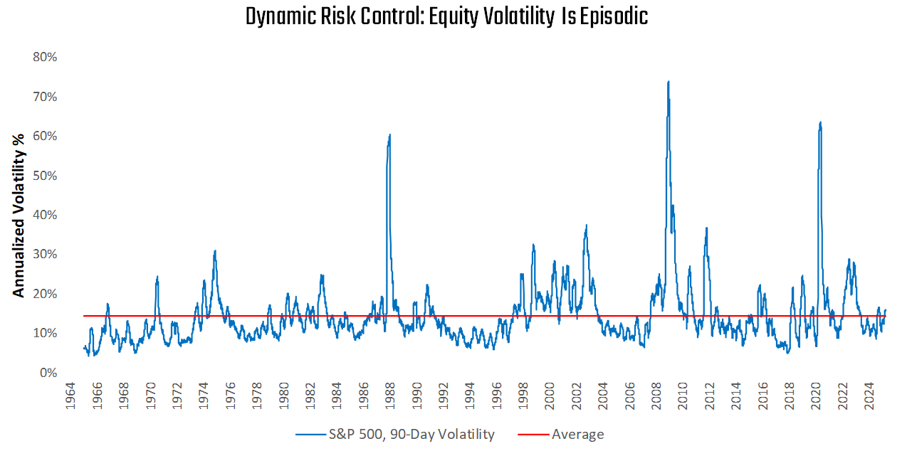
As we can see above, the long-term average annualized volatility of the S&P 500 is 15%. However, there are extremely large deviations from this average towards the upside, reaching as high as 70% during the 2008 Financial Crisis.

We think that simply matching equity market volatility during these periods exposes portfolios to unnecessary risk of loss. After all, while our signals may well provide outsized returns during these periods of high volatility, they run the risk of large drawdowns due to the locally elevated volatility levels. In our experience, most investors comfortable with taking equity-like risk are looking for a maximum drawdown profile of approximately 15%. When equity volatility spikes to over 30% annually, the odds of meeting these drawdown objectives decline dramatically. Furthermore, as the volatility of equities rises during these periods, so does the mechanical drag on compounded returns, also called volatility drag. This volatility drag reduces the cumulative risk-adjusted return over time.

Thus, considering both investor preferences and the effects of volatility drag, we think the best approach is to dynamically adjust risk over time based on signal strength and expected drawdown, with the explicit objective of a 15% maximum drawdown.

The further we are from this 15% drawdown threshold, the more unconstrained our portfolio risk-taking; the closer we get, the more we dial down risk. We want to take the most risk when we have the most signal, but we want to do that within reason. This dynamic process is different from traditional volatility targeting, which imposes a constant level of portfolio risk regardless of signal strength.

Mechanically, this type of process does not have return-boosting properties without leverage. However, it has the potential to increase risk-adjusted returns, particularly Calmar Ratios, as reflected in our simulations:

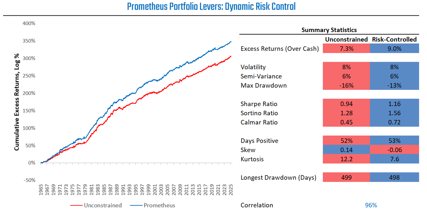
Above, we compare two portfolios. The first is an Unconstrained Portfolio, which takes our Beta Timing, Sector Selection, and Active Overlay and is always fully invested. The second is a Risk-Controlled Portfolio, which leverages our Dynamic Risk Control. For comparison, we scale down the volatility of the Unconstrained Portfolio to match that of the Risk Controlled Portfolio. The difference between the two portfolios is the benefit of our dynamic risk control. As we can see, risk control is beneficial to all risk metrics, but most beneficial to the Calmar Ratio. Further, this risk-control performs its explicit objective of maintaining a maximum drawdown of 15% over an extensive range of market environments, including Black Monday and the COVID-19 crash.

In conclusion, this dynamic version of risk-taking is significantly additive to portfolio performance. While dynamic risk control doesn’t directly enhance returns, it mitigates drawdowns and facilitates better risk-adjusted returns. Overall, Dynamic Risk Control allows us to press our edge when we feel strongly but tempers our bets to take risks consistent with investors' risk tolerance.

Prometheus S&P 500 Program: Simulation Study

Now that we have provided an in-depth analysis of the levers we use in our investment process, we dive into the details of our simulations. As systematic investors, we think a rigorous evaluation of how our systems performed over history is important to shape expectations and generate avenues for improvement. We think that stress-testing portfolios through a range of macroeconomic environments is paramount to this process. While most modern analysis occurs during the post-1996 period, we have invested significant time and effort into simulating macroconditions and markets going back to the 1960s. This gives us a much broader range of outcomes to stress-test our systems and understand their performance. We begin with the cumulative excess returns of our Prometheus S&P 500 Program versus its benchmark:

As we can see, the simulated path of the Prometheus S&P 500 Program has offered better returns, lower volatility and semi-variance, lower drawdowns in depth and duration, and better return to risk characteristics than the S&P 500 on a gross transaction costs basis across a wide range of macro environments.

For the purposes of examining this simulated performance more carefully, we zoom in on every decade in our simulation for a more granular understanding of the return stream. We begin our assessment of our simulated performance using an intuitive lens by breaking up our historically simulated performance into sub-samples. We look at 60 years of history, broken into six decade-long periods. These sub-samples include a very wide range of macroeconomic conditions, ranging from stagflation to quantitative easing and COVID-19. We visualize this below:

As we can see above, the Prometheus S&P 500 Program has performed in a manner consistent with its objectives over every recorded decade. It has done so during Stagflation (1960-1980), the Great Moderation (1985-2008), and the Dotcom. For informational purposes only. 9 Bubble (2000), the Financial Crisis (2008), Zero Interest Rate Policy & QE (2008-2015, 2020-2022), COVID-19 (220), and Fiscal Dominance (2020-Present). We share a comprehensive list of all the major macro shocks weathered over this period:

• 1965–1968: Vietnam War escalation and U.S. fiscal expansion

• 1969–1970: U.S. recession driven by Fed tightening

• 1971: Nixon ends gold convertibility (collapse of Bretton Woods)

• 1973: Yom Kippur War and OPEC oil embargo

• 1973–1974: Energy crisis and stagflation

• 1973–1975: U.S. recession and equity market decline

• 1979–1980: Second oil shock (Iranian Revolution)

• 1980–1982: Double-dip recession and rate spike

• 1981–1982: Latin American debt crisis

• 1985: Plaza Accord – coordinated dollar devaluation

• 1987: Black Monday – S&P 500 drops 22% in a single day

• 1989–1990: Peak of Japan’s asset bubble

• 1990–1991: U.S. recession and Gulf War

• 1992: European ERM crisis

• 1997: Asian Financial Crisis

• 1998: Russian default and LTCM collapse

• 2000–2002: Dot-com bust and bear market

• 2001: September 11 terrorist attacks

• 2002: Corporate scandals – Enron and WorldCom

• 2003: U.S. invasion of Iraq

• 2004–2005: Greenspan’s tightening cycle (“measured pace”)

• 2007–2009: Global Financial Crisis (GFC)

• 2008: Lehman Brothers collapse; systemic banking crisis

• 2009: Launch of QE1 (quantitative easing)

• 2010–2012: Eurozone sovereign debt crisis

• 2011: U.S. debt ceiling crisis and S&P downgrade

• 2013: Taper tantrum – bond yields spike on QE exit fears

• 2014: Global oil price collapse

• 2015: China devaluation and global growth fears

• 2016: Brexit referendum and Trump elected

• 2018: U.S.–China trade war escalation

• 2020: COVID-19 pandemic crash and lockdowns

• 2020–2021: Stimulus-driven recovery and asset inflation

• 2021–2022: Inflation surges to 40-year highs

• 2022: Fed begins aggressive rate hikes and QT

• 2023: Bank failures – SVB, Signature, Credit Suisse

• 2025: Tariff Shocks

This extremely wide array of macro market conditions allows us to build confidence in the durability of our systems.

The only decade when our simulated S&P 500 Program underperformed the index was during the 2015-2025 period. During this period the Prometheus S&P 500 Program generated a 10% annualized return at a 7% volatility, a risk and return profile entirely consistent with its objectives. Meanwhile, the S&P 500 Index generated a 12% annualized return at a 19% volatility.

On a risk-adjusted basis, the Prometheus S&P 500 Program generated a Sharpe Ratio of 1.0, while the S&P 500 Index generated a lower Sharpe Ratio of 0.63. However, the S&P 500 Index had a volatility of greater than 2x of the Prometheus S&P 500 Program, leading to higher gross returns despite meaningfully lower risk-adjusted returns. This lower gross return was primarily driven by our Dynamic Risk Control, which maintained a maximum drawdown of -13% during this period, despite three separate drawdowns in the 15-30% range for the S&P 500 Index. To capture how this relative underperformance was driven by our Dynamic Risk Control, we can look at our portfolio excluding the risk control lever, i.e., a fully invested portfolio with no cash position. This allows us to understand if there was any meaningful alpha decay during this period. We visualize the simulated path of the portfolio without our risk-control measures:

As we can see above, our systematic process would have outpaced the S&P 500 during this decade as well, but for our Dynamic Risk Control. However, it would have done so at significantly more risk than is consistent without objectives. With a Sharpe Ratio of 1 over this period, gross returns of 10%, and a maximum drawdown of 13%, the Prometheus S&P 500 performed in a manner consistent with its design. The 2015-2025 period has been one of the best recorded periods in history for the S&P 500, which we do not consider consistent with the long-term expected returns of the index. While our strategies are well-equipped to outperform even this environment by simply reducing its cash level to zero, we think that chasing high levels of volatility based on recency bias is inconsistent with meeting investors’ long-term needs. Overall, the Prometheus S&P 500 Program performed in line with its design, despite the lag during an exceptional period for performance for equities.

To further understand the durability of the systems underlying the Prometheus S&P 500 Program, we turn to cumulative returns conditional upon macro conditions. The objective of this assessment is to understand if there is a macroeconomic bias embedded in the program. We visualize the cumulative returns during growth accelerations, growth decelerations, inflation accelerations, and inflation decelerations below:

As we can see above, while there is modest variation in return paths, there is a generalized and consistent upwards drift across regimes. We capture this in tabular format relative to the benchmark:

Performance remains stable across regimes, particularly relative to the benchmark.

Thus far, we have looked at cumulative returns. Now, we turn to measures of risk, particularly the risk most impactful to investors' decision-making, i.e., drawdowns. To get a comprehensive understanding of our expected drawdown profile, we examine both drawdown depth and duration:

Our simulations show that the Prometheus S&P 500 Program has a significantly better drawdown profile than the benchmark in terms of both in-depth and duration. Per our mechanical design, the maximum drawdown has never exceeded the 15% threshold. Often, the strategy has generated positive performance during drawdown periods for the S&P 500, leading to relative outperformance.

In part, this relative performance is driven by strong risk control at the portfolio level. We show this using two perspectives. First, we visualize how realized portfolio volatility is controlled using measures of expected volatility before taking on new positions. This process allows the Prometheus S&P 500 Program to effectively control realized volatility, resulting in a historical maximum volatility of 12%. This realized volatility is significantly lower than the S&P 500 over time, and orders of magnitude less than the episodic spikes in equity volatility. We visualize these perspectives below:

Overall, combining modestly positive returns over time with volatility and drawdown control creates a comparatively stable return stream with limited exposure to equity market downside. As such, the Prometheus S&P 500 Program shows modest and consistent upside capture, with outperformance characteristics on the downside.

We examine one-year rolling returns to capture our systems' relative outperformance characteristics relative to the benchmark. Additionally, to isolate the value of our process during equity market drawdowns, we isolate the cumulative value of our program during S&P 500 Index drawdowns. We visualize this below:

As we can see in our rolling returns, the Prometheus S&P 500 Program generates a significantly less volatile return stream over time. It maintains reasonable upside to equity bull markets but avoids irrational exuberance while avoiding or mitigating large drawdowns. We see this downside mitigation in the program's cumulative performance during S&P 500 drawdowns, where, often through short S&P 500 and treasury exposure, index drawdowns are turned into gains.

Now that we have examined the return and risk characteristics of our simulated Prometheus S&P 500 Program, we can turn to the implementation hurdles. Particularly, we focus on transaction costs. Given our macro focus, the systems underlying the Prometheus S&P 500 Program move incrementally and gradually, controlling transaction costs:

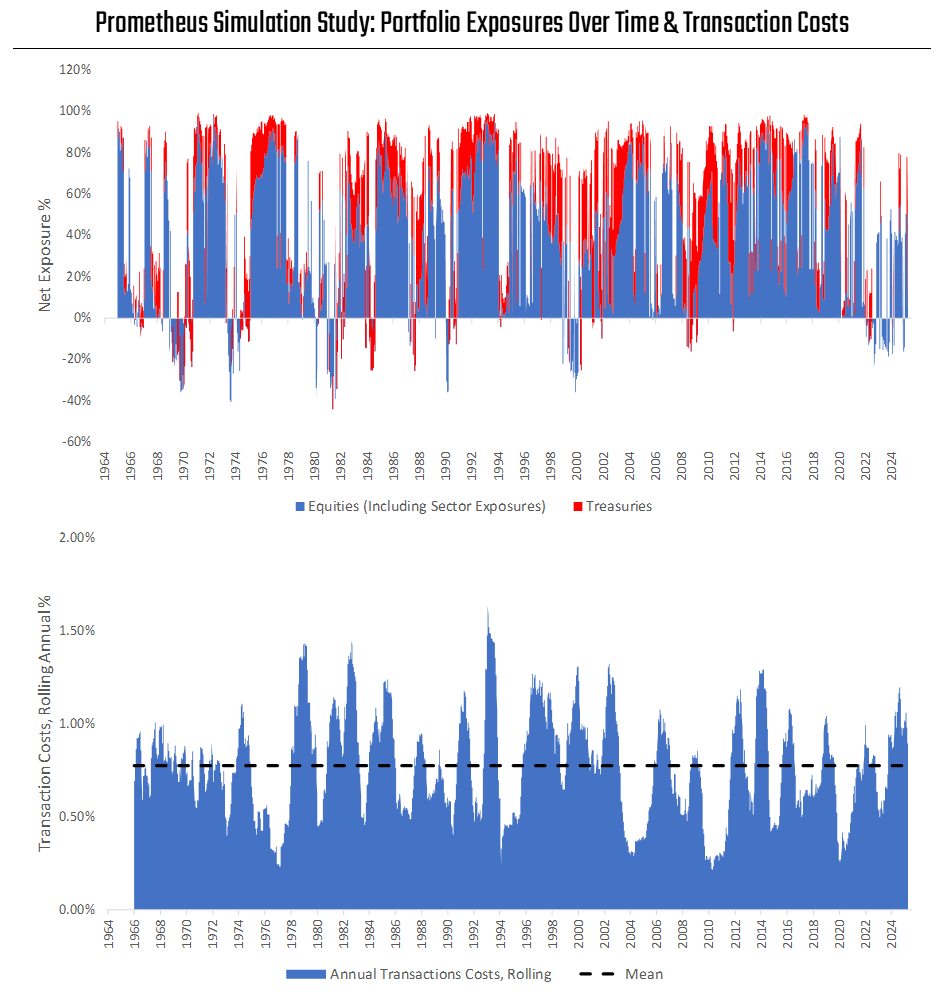
Above, we use relatively aggressive estimates of 0.1% of notional traded value to estimate transaction costs over time. Even with these aggressive estimates, annualized transaction costs reach 0.8% annually, dragging on returns minimally and maintaining a post-transactions cost Sharpe Ratio of 1.05.

Applications

The Prometheus S&P 500 Program leverages our proprietary process to improve equity exposure by carefully implementing a combination of Sector Selection, Beta Timing, Active Overlays, and Dynamic Risk Control. Given our systematic approach, we stress-test our process over a wide range of macroeconomic and market environments. Our simulations show that our approach weathers a wide variety of equity bull and bear markets, creating a stable return profile consistent with our expectations. Additionally, we have over a year of live signal history for the underlying signals we have been tracking internally, which shows these signals have operated in line with our expectations.

Going forward, this Prometheus S&P 500 Program will be available to all clients. The portfolio will rebalance once a week on Mondays, rotating between the ETFs SPY, XLI, XLE, XLK, XHB/ITB, TUA, TYA, and Cash. We note that the S&P 500 component will enter net short positions. The optimal way to express this view would be via S&P 500 Futures. Alternatively, using levered short ETFs such as SPXU or SPXS can achieve similar results. Finally, given the fact that net short equity exposure is relatively rare for the program, we think investors unable to use short exposure can benefit from simply moving total equity exposure to zero.

Every week, we will provide a note detailing the positions of the Prometheus S&P 500 Program and their expected volatility. This will allow investors to scale the portfolio to the volatility of their choosing, based upon their own circumstances. We show an illustrative example of this readout below:

As shown, positions and risk profiles will always be clearly stated. In addition to this programmatic readout, we will also provide color on the insights coming from each of our portfolio construction levers, i.e., Beta Timing, Sector Selection, Treasury Overlay, and Risk Control.

We show a sample of this report below:

Conclusions

The Prometheus S&P 500 Program has been live since March 2025, only to be immediately met by extremely high tariff-induced market volatility, which it has weathered in a manner entirely consistent with our simulations. While S&P 500 Index volatility soared, resulting in a maximum drawdown of 18%, the Prometheus S&P 500 never exceeded a 10% drawdown, and is at a 3% drawdown at the time of writing.

The Prometheus S&P 500 Program reflects our recognition that the S&P 500 is likely to remain an integral part of investor portfolios for the foreseeable future. As such, we think it’s our job to add an edge to those portfolios. We believe that with reliable, durable, and uncorrelated alpha, it is possible to outperform the equity market significantly over a full investment cycle. Crucially, we don’t think it is possible to outperform every week, month, or even year. However, with a consistent and disciplined approach, we think it is possible to harness most of the upside in equities while ameliorating or avoiding the downside. We think the outperformance generated through the successful implementation of this process will materialize over the course of a full investment cycle.

These views are validated by extremely rigorous back testing and by our live experience over the years of using the signals driving this portfolio. No strategy is without its risk, but with durable signals, a long-term exposure to equity beta, diversification via treasury exposure, and clearly defined maximum loss objective- we think the Prometheus S&P 500 Program offers a strong tool in the toolkit of active investors at the least and potentially even a replacement for passive S&P 500 exposure entirely where appropriate. For now, the portfolio will be provided as a model portfolio, but in time, we intend to explore the tax benefits of providing this within an ETF wrapper.

We look forward to continuing our mission to democratize access to institutional-quality research and insights to the investing public. Another step towards the democratization of finance.

Until next time.